
Historical SI Ampere and Parallel Wires: HSC Physics
Learn how the force between parallel current-carrying wires connected Newton's third law to the former SI definition of the ampere.
Imagine being told to define exactly what “1 ampere” means, but you’re not allowed to use an ammeter. For much of the twentieth century, the official answer was wonderfully physical: put two ideal wires beside each other, run current through them, and define the ampere by the tiny magnetic force they exert on each other.
Before seeing the details, predict this: if the two currents flow in the same direction, should the wires attract or repel? A reasonable guess is “repel”, because we often associate magnetic things with pushing apart. The actual result is the opposite. Parallel currents in the same direction attract; currents in opposite directions repel.
That force became important enough that, from 1948 until the revised SI took effect on 20 May 2019, it sat at the heart of the definition of the ampere. :chatgpt-content-reference{index=”0″}
01Why two currents can push on each other
Start with one long, straight wire carrying current \(I_1\).
That current produces a magnetic field around the wire. At a perpendicular distance \(r\), the field strength is
\[ B_1=\frac{\mu_0 I_1}{2\pi r} \]
where:
- \(B_1\) is the magnetic field produced by wire 1, in tesla (T),
- \(\mu_0\) is the permeability of free space,
- \(I_1\) is the current in wire 1, in amperes (A), and
- \(r\) is the perpendicular distance from wire 1, in metres (m).
Now place wire 2 parallel to wire 1.
Wire 2 sits inside the magnetic field created by wire 1. A current-carrying conductor in an external magnetic field experiences the motor-effect force
\[ F=I_2LB\sin\theta \]
where \(I_2\) is the current in wire 2, \(L\) is the length considered, and \(\theta\) is the angle between the current and the magnetic field.
At wire 2, the circular magnetic field from wire 1 is perpendicular to wire 2. Therefore \(\theta=90^\circ\), so \(\sin\theta=1\).
Substituting the field from wire 1 gives
\[ F =I_2L\left(\frac{\mu_0 I_1}{2\pi r}\right) \]
and hence
\[ \frac{F}{L}=\frac{\mu_0 I_1I_2}{2\pi r} \]
This is the key parallel-wire relationship.
The force per unit length increases when either current increases. It decreases as the separation increases.
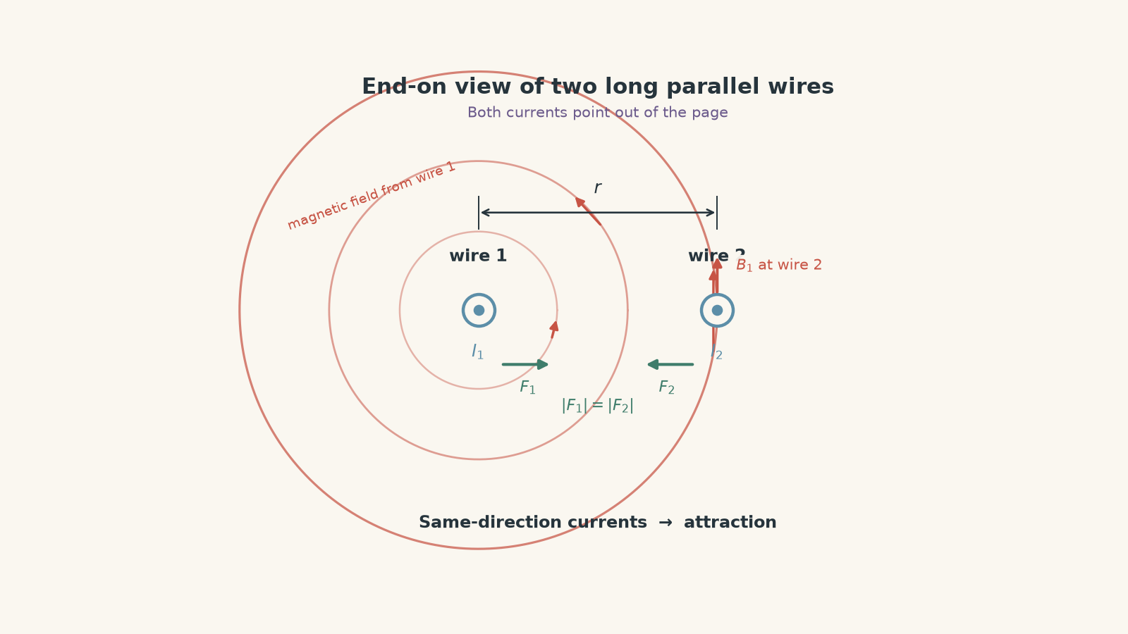
If the direction part still feels slippery, the motor-effect direction rules are worth reviewing separately. The magnitude equation does not tell you whether the force is attractive or repulsive.
02Why currents in the same direction attract
Suppose both currents point upwards.
Use the right-hand grip rule around wire 1. At the location of wire 2, its magnetic field points in a definite direction perpendicular to the wires. Applying the motor-effect force rule to wire 2 gives a force towards wire 1.
Now swap the roles.
Wire 2 creates its own magnetic field at wire 1. That field produces a force on wire 1 towards wire 2.
So the wires attract.
If one current is reversed, both force directions reverse. The wires then repel.
A useful decision rule is:
| Current directions | Interaction |
|---|---|
| Same direction | Attraction |
| Opposite directions | Repulsion |
Don’t memorise this as an isolated fact if you can avoid it. It follows from “one wire makes the field; the other current experiences the force”.
Worked example: Force between two parallel wires
Two long parallel wires are \(0.12\text{ m}\) apart. They carry currents of \(3.0\text{ A}\) and \(5.0\text{ A}\) in opposite directions. Calculate the force acting on a \(0.40\text{ m}\) length of either wire.
Step 1
\[ F=\frac{\mu_0 I_1I_2L}{2\pi r} \]
For HSC calculations, take
\[ \mu_0\approx4\pi\times10^{-7}\text{ N A}^{-2} \]
Step 2
\[ \begin{aligned} F &=\frac{(4\pi\times10^{-7})(3.0)(5.0)(0.40)} {2\pi(0.12)}\\ &=1.0\times10^{-5}\text{ N} \end{aligned} \]
Step 3
The currents are opposite, so the wires repel.
Therefore each \(0.40\text{ m}\) section experiences a force of
\[ 1.0\times10^{-5}\text{ N} \]
directed away from the other wire.
That force is tiny, but tiny is enough if your measuring apparatus is good.
03Where Newton’s third law appears
Look again at
\[ \frac{F}{L}=\frac{\mu_0 I_1I_2}{2\pi r} \]
Notice something important: it does not matter whether you call one current \(I_1\) or \(I_2\). The product \(I_1I_2\) is the same.
So, for the ideal two-wire system, the magnitude of the force on wire 1 due to wire 2 equals the magnitude of the force on wire 2 due to wire 1.
The directions are opposite.
That is exactly what Newton’s third law requires here:
\[ \vec F_{1\leftarrow2}=-\vec F_{2\leftarrow1} \]
There is a common trap hiding here. Equal forces do not mean equal accelerations.
If one wire has twice the mass per metre of the other, the two forces can be equal while the lighter wire accelerates twice as much, because
\[ a=\frac{F}{m} \]
Newton’s third law concerns forces, not motions.
There is also a more advanced limitation worth knowing. In general electromagnetic systems, fields themselves can carry momentum. You should not use this simple two-wire argument as a shortcut for every changing electromagnetic situation. For the steady, ideal parallel-current problem used here, however, the mechanical forces are equal and opposite.
04The measurement problem that led to the old ampere
A unit is not very useful if laboratories cannot agree on what it means.
Electrical measurements once depended on practical artefacts and agreed procedures. A more fundamental approach was to connect electrical current to mechanical quantities such as force, distance, and length.
The parallel-wire model offered exactly that connection.
Picture the ideal arrangement in spatial order:
- Two straight conductors run beside each other.
- Their centre lines are \(1\text{ m}\) apart.
- They are assumed to be infinitely long.
- Their circular cross-sections are assumed negligible.
- They sit in vacuum.
- The same constant current magnitude is maintained in the conductors.
- The magnetic interaction produces a measurable force between them.
The historical definition adopted in 1948 specified that a current of one ampere would produce a force per unit length of
\[ 2\times10^{-7}\text{ N m}^{-1} \]
for this ideal \(1\text{ m}\) separation. :chatgpt-content-reference{index=”1″}
It was not saying that every laboratory should somehow obtain two genuinely infinite, infinitely thin wires. Those conditions define an ideal physical model.
That distinction matters.
05A scale estimate: how small was the defining force?
Put \(I_1=I_2=1\text{ A}\) and \(r=1\text{ m}\) into the wire-force equation:
\[ \begin{aligned} \frac{F}{L} &=\frac{(4\pi\times10^{-7})(1)(1)} {2\pi(1)}\\ &=2\times10^{-7}\text{ N m}^{-1} \end{aligned} \]
So a one-metre section would experience a force of only
\[ F=2\times10^{-7}\text{ N}. \]
To get a feel for that number, ask what mass would have the same weight near Earth’s surface.
Using \(F=mg\),
\[ \begin{aligned} m&=\frac{F}{g}\\ &=\frac{2\times10^{-7}}{9.81}\\ &\approx2.0\times10^{-8}\text{ kg} \end{aligned} \]
That is about \(20\) micrograms of mass.
So the old definition connected one ampere to a mechanically measurable effect, but the effect was extremely small.
06The clever connection to \(\mu_0\)
Now comes the part that is easy to miss.
The old definition did more than define the ampere. It also made the value of \(\mu_0\) exact.
Take
\[ \frac{F}{L}=\frac{\mu_0I_1I_2}{2\pi r}. \]
For the defining situation,
\[ I_1=I_2=1\text{ A}, \qquad r=1\text{ m}, \qquad \frac FL=2\times10^{-7}\text{ N m}^{-1}. \]
Rearrange for \(\mu_0\):
\[ \begin{aligned} \mu_0 &=\frac{2\pi r(F/L)}{I_1I_2}\\ &=2\pi(1)(2\times10^{-7})\\ &=4\pi\times10^{-7}\text{ N A}^{-2}. \end{aligned} \]
Under the former definition, that value was exact because the definition of the ampere had been constructed to make it so.
That is very different from merely measuring \(\mu_0\) and finding something close to \(4\pi\times10^{-7}\).
07But nobody has an infinite wire
Here is the obvious flaw in the ideal arrangement: infinite wires do not fit comfortably in a laboratory.
Neither do wires with literally negligible thickness.
Real conductors also have finite length, supports, connections, and surrounding equipment. Those features alter the magnetic forces slightly from the perfect ideal model.
So practical force measurements used current balances and carefully designed conductor arrangements rather than physically reproducing the definition word for word. In a current balance, magnetic forces between conductors or coils can be compared with a known mechanical force on a balance. The geometry must then be understood accurately enough to connect the real apparatus back to the ideal electromagnetic relationship. NIST describes, for example, a Kelvin balance that compared magnetic forces between coils with mechanical forces from masses. :chatgpt-content-reference{index=”2″}
This is a useful historical lesson: a definition and a practical realisation of that definition are not necessarily the same object.
The definition says what the unit means. Metrology tells you how to realise it accurately.
Worked example: Inferring an unknown current
Two long parallel wires are \(4.0\text{ cm}\) apart. Wire 1 carries \(5.0\text{ A}\). The measured force per unit length between the wires is \(3.0\times10^{-4}\text{ N m}^{-1}\). Find the magnitude of the current in wire 2.
Step 1
\[ r=4.0\text{ cm}=0.040\text{ m} \]
Step 2
\[ \frac FL=\frac{\mu_0I_1I_2}{2\pi r} \]
Rearrange for \(I_2\):
\[ I_2=\frac{2\pi r(F/L)}{\mu_0I_1} \]
Step 3
\[ \begin{aligned} I_2 &=\frac{2\pi(0.040)(3.0\times10^{-4})} {(4\pi\times10^{-7})(5.0)}\\ &=12\text{ A} \end{aligned} \]
The second current has magnitude \(12\text{ A}\).
Notice that the force measurement alone gives the magnitude of \(I_2\). To determine whether its current points in the same or opposite direction to \(I_1\), you would also need to know whether the wires attract or repel.
08Why the ampere definition changed in 2019
The force definition had a strong physical idea behind it, but its ideal geometry was awkward to realise directly.
Modern metrology also gained access to electrical standards based on quantum physics. So the revised SI changed what was treated as exact.
Since 20 May 2019, the ampere has been defined by fixing the elementary charge \(e\) to exactly
\[ e=1.602\,176\,634\times10^{-19}\text{ C}. \]
Because \(1\text{ C}=1\text{ A\,s}\), this ties electric current directly to charge transferred per unit time. :chatgpt-content-reference{index=”3″}
In rate form,
\[ I=\frac{\Delta q}{\Delta t}. \]
A current of \(1\text{ A}\) therefore corresponds to a charge-flow rate of about
\[ \frac{1}{1.602\,176\,634\times10^{-19}} \approx6.2415\times10^{18} \]
elementary charges per second.
Do not read that as “electrons must move through a metal wire at \(6.24\times10^{18}\) metres per second” or anything remotely like that. It is a count of charge crossing a chosen surface per second, not the speed of individual electrons.
The modern definition fixes \(e\), not \(\mu_0\). As a result, \(\mu_0\) is now a quantity that must, in principle, be determined experimentally rather than having the exact defined value \(4\pi\times10^{-7}\text{ N A}^{-2}\). The numerical difference is far below the precision relevant to ordinary HSC calculations, so using \(4\pi\times10^{-7}\) remains an excellent approximation at this level. :chatgpt-content-reference{index=”4″}
| Former SI | Current SI |
|---|---|
| Ampere tied to force between ideal parallel conductors | Ampere tied to the fixed elementary charge \(e\) |
| \(\mu_0=4\pi\times10^{-7}\text{ N A}^{-2}\) exactly | \(e=1.602\,176\,634\times10^{-19}\text{ C}\) exactly |
| Force experiment helped realise current | Precisely realised current can instead be used to investigate electromagnetic constants |
| Ideal infinite-wire geometry built into the definition | Fundamental constant built into the definition |
Nothing dramatic happened to electrical devices on 20 May 2019. A laboratory current did not suddenly jump because the wording changed. The revised SI was designed to preserve continuity while changing the underlying definition.
09What HSC students should take from the history
The historical ampere gives you a reason for learning the force-between-wires equation. It was not merely an equation sitting on a formula sheet. It once helped define one of the SI base units.
It also connects several HSC ideas that are often learned separately:
- a current produces a magnetic field,
- another current in that field experiences a force,
- the interaction gives equal and opposite forces in the ideal two-wire system,
- the magnitude depends on \(I_1I_2/r\),
- a measurable mechanical force can be used to infer an electrical quantity, and
- changing a scientific definition can change which constant is treated as exact without changing the underlying physics.
For more calculation practice with the relationship itself, see Force Between Parallel Current-Carrying Wires.
10Questions and solutions
Question 1
Two long parallel wires are \(0.15\text{ m}\) apart and carry currents of \(4.0\text{ A}\) and \(6.0\text{ A}\) in the same direction.
Calculate the force acting on a \(0.80\text{ m}\) section of either wire and state its direction.
Solution 1
The force on each \(0.80\text{ m}\) section is \(2.56\times10^{-5}\text{ N}\), directed towards the other wire.
Use
\[ F=\frac{\mu_0I_1I_2L}{2\pi r}. \]
Substitute:
\[ \begin{aligned} F &=\frac{(4\pi\times10^{-7})(4.0)(6.0)(0.80)} {2\pi(0.15)}\\ &=2.56\times10^{-5}\text{ N}. \end{aligned} \]
The currents flow in the same direction, so the interaction is attractive.
A tempting mistake is to find the correct magnitude and then assume the force points “along the magnetic field”. It does not. The force direction comes from the interaction between the current direction and the magnetic field, not from the magnetic field direction alone.
Question 2
Two parallel wires are \(0.080\text{ m}\) apart. Wire A carries \(10\text{ A}\), while wire B carries an unknown current in the opposite direction.
The force per unit length is \(5.0\times10^{-4}\text{ N m}^{-1}\).
- Find the current in wire B.
- Wire A has mass per unit length \(1.0\times10^{-2}\text{ kg m}^{-1}\), while wire B has mass per unit length \(2.0\times10^{-2}\text{ kg m}^{-1}\). If both wires are released sideways and other forces are ignored, find each wire’s initial acceleration.
- Explain why the accelerations are different without violating Newton’s third law.
Solution 2
Wire B carries \(20\text{ A}\). Wire A initially accelerates at \(5.0\times10^{-2}\text{ m s}^{-2}\), while wire B accelerates at \(2.5\times10^{-2}\text{ m s}^{-2}\), in opposite directions.
For the current,
\[ \frac FL=\frac{\mu_0I_AI_B}{2\pi r}. \]
Therefore
\[ \begin{aligned} I_B &=\frac{2\pi r(F/L)}{\mu_0I_A}\\ &=\frac{2\pi(0.080)(5.0\times10^{-4})} {(4\pi\times10^{-7})(10)}\\ &=20\text{ A}. \end{aligned} \]
Because the currents are opposite, the wires repel.
For wire A, consider one metre of wire. The force is \(5.0\times10^{-4}\text{ N}\), and its mass is \(1.0\times10^{-2}\text{ kg}\).
\[ \begin{aligned} a_A &=\frac{F}{m}\\ &=\frac{5.0\times10^{-4}} {1.0\times10^{-2}}\\ &=5.0\times10^{-2}\text{ m s}^{-2}. \end{aligned} \]
For one metre of wire B,
\[ \begin{aligned} a_B &=\frac{5.0\times10^{-4}} {2.0\times10^{-2}}\\ &=2.5\times10^{-2}\text{ m s}^{-2}. \end{aligned} \]
The tempting conclusion is that different accelerations must mean different forces. That confuses Newton’s second and third laws.
Newton’s third law says the interaction forces are equal in magnitude and opposite in direction. Newton’s second law says the resulting acceleration also depends on mass. Wire B has twice the mass per unit length, so its acceleration is half as large.
Question 3
Three long parallel wires, A, B, and C, lie along a straight horizontal line.
Wire B is \(0.10\text{ m}\) to the right of A. Wire C is another \(0.20\text{ m}\) to the right of B.
A and B carry currents of \(4.0\text{ A}\) and \(3.0\text{ A}\), respectively, in the same direction.
- Determine the magnitude and direction of the current in C required for the net magnetic force on B to be zero.
- If the direction of current B is then reversed while A and C remain unchanged, is the net force on B still zero? Explain without repeating the full calculation.
Solution 3
Wire C must carry \(8.0\text{ A}\) in the same direction as A and B. Reversing only the current in B still gives zero net force on B, although both individual force directions reverse.
The force per unit length on B due to A is
\[ \frac{F_{BA}}L =\frac{\mu_0I_AI_B}{2\pi r_{AB}}. \]
A and B carry current in the same direction, so A attracts B towards the left.
For zero net force, C must pull B equally strongly towards the right. Therefore C must carry current in the same direction as B.
Set the magnitudes equal:
\[ \frac{\mu_0I_AI_B}{2\pi r_{AB}} = \frac{\mu_0I_CI_B}{2\pi r_{BC}}. \]
Cancel the common factors:
\[ \frac{I_A}{r_{AB}} = \frac{I_C}{r_{BC}}. \]
So
\[ \begin{aligned} I_C &=I_A\frac{r_{BC}}{r_{AB}}\\ &=(4.0)\frac{0.20}{0.10}\\ &=8.0\text{ A}. \end{aligned} \]
Now reverse only \(I_B\).
The magnitude of each interaction still contains the same product of current magnitudes, so both magnitudes are unchanged. However, B now carries current opposite to both A and C, so both attractions become repulsions.
A now pushes B to the right, while C pushes B to the left. The two forces are still equal.
The trap is to think that reversing B must destroy the balance. It reverses both forces acting on B, so their vector sum remains zero.
Question 4
Imagine a modern experiment using two extremely long parallel conductors separated by exactly \(1.000000000\text{ m}\). Each current has been independently realised as \(1.000000000\text{ A}\) using the current SI definition.
Suppose, after all experimental corrections have been made, the measured force per unit length is hypothetically
\[ 2.000000004\times10^{-7}\text{ N m}^{-1}. \]
- Use the measurement to infer \(\mu_0\).
- Compare it with \(4\pi\times10^{-7}\text{ N A}^{-2}\).
- Explain why the interpretation of such an experiment is fundamentally different under the current SI from what it would have been under the former force-based ampere definition.
Solution 4
The hypothetical result gives
\[ \mu_0=4.000000008\pi\times10^{-7}\text{ N A}^{-2}, \]
which is larger than \(4\pi\times10^{-7}\text{ N A}^{-2}\) by a fractional amount of \(2\times10^{-9}\).
Rearrange the parallel-wire equation:
\[ \mu_0 = \frac{2\pi r(F/L)}{I_1I_2}. \]
Substitute the stated values:
\[ \begin{aligned} \mu_0 &= \frac{2\pi(1.000000000) (2.000000004\times10^{-7})} {(1.000000000)(1.000000000)}\\ &=4.000000008\pi\times10^{-7}\text{ N A}^{-2}. \end{aligned} \]
Compare this with the familiar value:
\[ 4.000000008\pi\times10^{-7} = \left(4\pi\times10^{-7}\right) (1.000000002). \]
So the fractional difference is
\[ 2\times10^{-9}. \]
Under the current SI, the elementary charge \(e\) is fixed exactly. The ampere can therefore be realised independently of the parallel-wire force law, and an accurate force experiment can be interpreted as a measurement of \(\mu_0\).
Under the former definition, that logic ran the other way. The force relationship was part of what established the ampere, and \(\mu_0=4\pi\times10^{-7}\text{ N A}^{-2}\) followed exactly from the definition.
So, before 2019, a discrepancy would not have meant “we have measured a slightly different value of \(\mu_0\)” within that SI framework. It would instead have pointed towards imperfect current realisation, imperfect geometry, measurement error, or an unresolved problem with the experiment.
The tempting route is to treat a familiar numerical constant as if it has always had the same logical status. It has not. The electromagnetic physics remains the same, but the definition tells us which quantity is taken as exact and which can be measured.
Question 5
Consider the ideal historical geometry: two infinitely long, negligible-thickness wires are \(1\text{ m}\) apart in vacuum, and the measured force per unit length is exactly
\[ 2\times10^{-7}\text{ N m}^{-1}. \]
A student argues:
“Newton’s third law says the two forces are equal, so the two currents must also be equal. Therefore each current must be \(1\text{ A}\).”
Analyse the claim in each situation below.
- The two wires have independent current sources.
- The two wires are connected in series, so the same steady current must pass through both.
- Explain what Newton’s third law actually contributes to the reasoning, and what it does not.
- Under the current SI, suppose the series current is already independently known to be exactly \(1\text{ A}\). What could the wire-force measurement then tell you?
Solution 5
With independent current sources, the measurement does not prove that each current is \(1\text{ A}\); it fixes only their product. With the wires in series, the added constraint \(I_1=I_2\) allows the historical result to identify the common current as \(1\text{ A}\). Newton’s third law establishes equal and opposite interaction forces, not equal currents. Under the current SI, an independently known \(1\text{ A}\) series current turns the force experiment into a measurement of \(\mu_0\).
Start with
\[ \frac FL=\frac{\mu_0I_1I_2}{2\pi r}. \]
Using the former exact value
\[ \mu_0=4\pi\times10^{-7}\text{ N A}^{-2}, \]
together with \(r=1\text{ m}\) and
\[ \frac FL=2\times10^{-7}\text{ N m}^{-1}, \]
gives
\[ \begin{aligned} 2\times10^{-7} &= \frac{(4\pi\times10^{-7})I_1I_2} {2\pi}\\ &=2\times10^{-7}I_1I_2. \end{aligned} \]
Therefore
\[ I_1I_2=1\text{ A}^2. \]
That does not require
\[ I_1=I_2=1\text{ A}. \]
For example,
\[ I_1=0.50\text{ A}, \qquad I_2=2.0\text{ A} \]
produces the same product and therefore the same force magnitude.
This is the central trap. Equal interaction forces do not tell you that the quantities causing the interaction must themselves be equal.
Newton’s third law gives
\[ |\vec F_{1\leftarrow2}| = |\vec F_{2\leftarrow1}| \]
regardless of whether the two currents have equal magnitudes. The symmetry also appears directly in the factor \(I_1I_2\).
Now add the series condition.
For steady current through two series conductors,
\[ I_1=I_2=I. \]
The force equation then gives
\[ I^2=1\text{ A}^2. \]
Taking the current magnitude,
\[ I=1\text{ A}. \]
Only now can you conclude that the common current is one ampere. The decisive extra information was not Newton’s third law. It was the circuit constraint that the same current passes through both series conductors.
Under the current SI, reverse the logic again. If \(I=1\text{ A}\) is already established independently from the charge-based definition, then
\[ \mu_0=\frac{2\pi r(F/L)}{I^2}. \]
The parallel-wire apparatus is no longer needed to tell you what one ampere means. Instead, known current and measured force can tell you about \(\mu_0\).
That reversal is the real historical connection: the force law did not stop being true when the SI changed. What changed was which side of the equation served as the standard and which side became something to determine experimentally.
The next useful step is to carry the same motor-effect idea from one straight wire to conductors at other angles. That is where the \(\sin\theta\) term stops quietly being \(1\), and the conditions for maximum and zero motor-effect force become important.