
Induction from Moving Magnets and Conductors: HSC Physics
Learn how relative motion between magnets, wires, coils, and plates can generate an emf, and when motion produces no net induction. Includes worked examples, misconceptions, and challenging HSC-style questions.
Push a bar magnet towards a coil and a voltage appears across the coil. Hold the magnet still and push the coil towards the magnet instead. What happens?
Predict before reading on: if the relative motion is the same, should the induced emf be different because the magnet is now stationary?
In the usual HSC situation, no. The same change in magnetic flux through the coil gives the same induced emf. But that does not mean that “anything moving near a magnetic field produces a voltage”. A wire can move through a field and develop an emf, while an entire closed loop can move through that same field and have zero net emf.
That apparent contradiction is the important idea. Motion matters only when it changes the magnetic flux linked with a circuit, or when charges inside a conductor move through a magnetic field in a way that separates them.
01Start with what the coil actually notices
Imagine a coil sitting in front of the north pole of a bar magnet.
Move the magnet towards the coil. The magnetic field through the coil gets stronger, so the magnetic flux through the coil changes. Move the magnet away, and the flux changes in the opposite direction.
Now put the magnet and coil on the same skateboard and move the whole setup across the room without changing their separation or orientation. They are both moving quickly relative to the floor, but the coil keeps experiencing essentially the same magnetic field.
No changing flux means no induced emf from that motion.
This gives us a much better rule than “movement causes induction”:
Look for a change in the magnetic flux linked with the conductor.
Sometimes the magnet moves. Sometimes the conductor moves. Sometimes both move. Sometimes neither moves, but the magnetic field itself changes.
The useful question is always: what is changing from the conductor’s point of view?
02Magnetic flux is the quantity that ties the cases together
For a flat area in a uniform magnetic field, magnetic flux is
\[
\Phi = BA\cos\theta
\]
where:
- \(\Phi\) is magnetic flux, measured in webers (\(\text{Wb}\)),
- \(B\) is magnetic field strength, measured in teslas (\(\text{T}\)),
- \(A\) is the area enclosed by the loop, measured in square metres (\(\text{m}^2\)), and
- \(\theta\) is the angle between the magnetic field and the normal to the area.
The normal is an imaginary line perpendicular to the plane of the loop.
That last detail catches plenty of students. If the field passes straight through the face of the coil, then \(\theta=0^\circ\), not \(90^\circ\), so the flux is maximum.
For a real bar magnet, the field usually isn’t perfectly uniform across the whole coil. The expression \(\Phi=BA\cos\theta\) is therefore a model using an appropriate uniform or average field. The underlying idea remains the same: flux measures how much magnetic field passes through the loop in the relevant direction.
A coil with \(N\) turns has \(N\) times as much flux linkage:
\[
\text{flux linkage}=N\Phi
\]
Faraday’s law then relates a change in that flux linkage to induced emf:
\[
\varepsilon=-N\frac{\Delta\Phi}{\Delta t}
\]
where:
- \(\varepsilon\) is the induced emf in volts (\(\text{V}\)),
- \(N\) is the number of turns,
- \(\Delta\Phi\) is the change in flux through one turn, and
- \(\Delta t\) is the time over which the change occurs.
The minus sign records the direction described by Lenz’s law: the induced effect opposes the change that produced it.
If you need more practice using the equation itself, see Faraday’s Law for HSC Physics: Calculating Induced EMF.
03Moving a magnet towards a coil
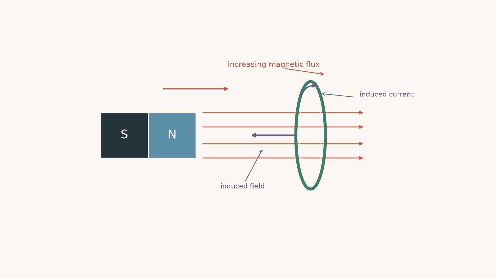
Suppose the north pole of a magnet approaches a stationary coil.
As the magnet gets closer:
- the magnetic field at the coil becomes stronger,
- the magnetic flux through the coil changes,
- an emf is induced, and
- if the circuit is closed, an induced current flows.
The faster the magnet moves, the faster the flux changes. That produces a larger magnitude of emf.
The effect also becomes larger if the coil has more turns because each turn experiences the changing flux.
What if the magnet stops halfway towards the coil?
The field through the coil may now be quite strong, but once the magnet has stopped, the flux is no longer changing. The induced emf falls to zero.
This is an important distinction:
A large magnetic flux does not necessarily produce an emf. A changing magnetic flux does.
A coil can sit in an enormous constant field and have no induced emf at all.
Worked example: A magnet increases the field through a coil
A 400-turn coil has an area of \(3.0\times10^{-3}\text{ m}^2\). Its area normal is parallel to the magnetic field. As a magnet approaches, the average magnetic field through the coil increases from \(0.020\text{ T}\) to \(0.065\text{ T}\) in \(0.15\text{ s}\).
Calculate the magnitude of the average induced emf.
Step 1
The area and orientation stay constant. Only \(B\) changes.
Since \(\theta=0^\circ\),
\[
\Phi=BA
\]
so
\[
\Delta\Phi=A\Delta B
\]
Step 2
\[
\begin{aligned}
\Delta B&=0.065-0.020\\
&=0.045\text{ T}\\[4pt]
\Delta\Phi&=(3.0\times10^{-3})(0.045)\\
&=1.35\times10^{-4}\text{ Wb}
\end{aligned}
\]
Step 3
For the magnitude,
\[
\begin{aligned}
|\varepsilon|
&=N\frac{|\Delta\Phi|}{\Delta t}\\
&=400\left(\frac{1.35\times10^{-4}}{0.15}\right)\\
&=0.36\text{ V}
\end{aligned}
\]
The average induced emf is \(0.36\text{ V}\).
The result means the approaching magnet changes the flux linkage quickly enough to produce an average potential difference of \(0.36\text{ V}\) around the coil. The direction would require information about the magnetic field direction and can then be found using Lenz’s law.
04Moving the coil instead of the magnet
Now keep the magnet fixed and move the coil towards it.
The coil enters regions of progressively stronger magnetic field, so its magnetic flux again changes. An emf is induced.
If the magnet-moving and coil-moving experiments produce exactly the same flux-versus-time behaviour, they produce the same emf-versus-time behaviour.
This is why relative motion is often a useful way to think.
But there is a limit to that shortcut. Saying “there is relative motion” isn’t enough by itself. You still need to check whether the flux linkage actually changes.
For example:
| Situation | Induced effect? | Reason |
|---|---|---|
| Magnet approaches stationary coil | Yes | \(B\) through the coil changes |
| Coil approaches stationary magnet | Yes | Coil moves through regions of different \(B\) |
| Magnet and coil move together at fixed separation | No, in the idealised setup | Flux linkage stays constant |
| Coil rotates in a uniform field | Usually yes | \(\theta\) changes |
| Coil changes area in a field | Usually yes | \(A\) changes |
| Closed loop translates entirely inside a uniform field | No net emf | \(B\), \(A\), and \(\theta\) stay constant |
The last case deserves special attention.
05A moving wire can develop an emf even in a steady field
Take a straight metal rod and move it sideways through a uniform magnetic field.
The free electrons in the rod are moving with the rod. A moving charge in a magnetic field experiences a magnetic force.
Its magnitude is
\[
F=qvB\sin\alpha
\]
where:
- \(F\) is the magnetic force in newtons (\(\text{N}\)),
- \(q\) is the charge in coulombs (\(\text{C}\)),
- \(v\) is the charge’s speed through the field in metres per second (\(\text{m s}^{-1}\)),
- \(B\) is magnetic field strength, and
- \(\alpha\) is the angle between the velocity and magnetic field.
In the common HSC arrangement, the rod moves perpendicular to the field, and the magnetic force pushes positive and negative charges towards opposite ends of the rod.
That charge separation creates a potential difference.
If the rod has length \(\ell\), and the rod, its velocity, and the magnetic field are mutually perpendicular, the motional emf is
\[
\varepsilon=B\ell v
\]
More generally, for the standard rod orientation,
\[
\varepsilon=B\ell v\sin\alpha
\]
where \(\alpha\) is the angle between \(v\) and \(B\).
Notice what has changed from the magnet-and-coil case. A stationary coil near a moving magnet experiences an induced electric field because the magnetic field through it changes. In the moving-rod case, charges are physically being carried through a magnetic field and experience magnetic force.
At HSC level, these situations are brought together by electromagnetic induction and Faraday’s law.
06Put the moving rod on rails
A lone rod develops charge separation between its ends. To obtain a continuous current, connect the rod into a complete conducting circuit.
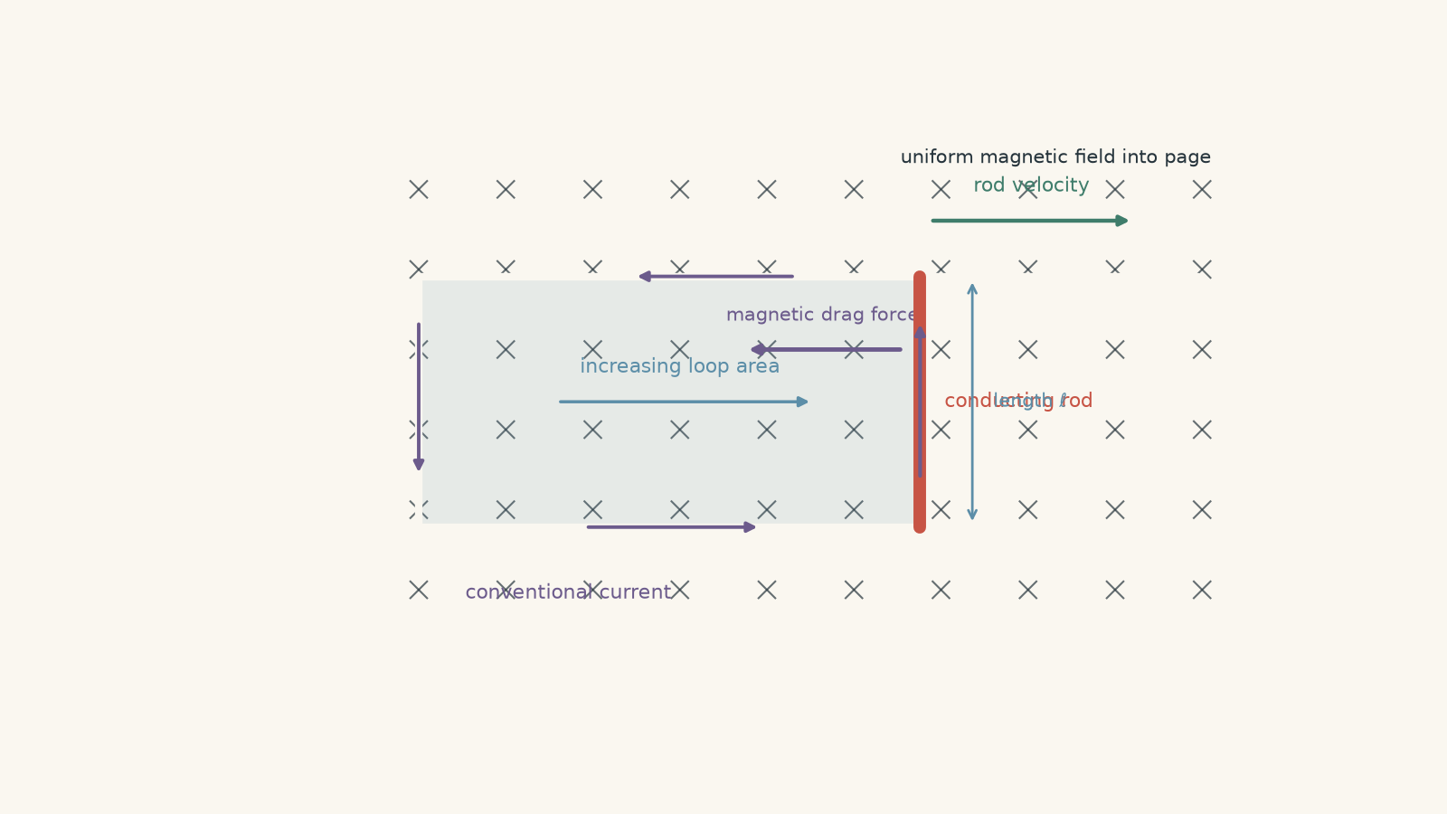
A standard arrangement uses two stationary rails joined at one end, with a conducting rod sliding along them.
As the rod moves:
- the area of the circuit increases,
- the magnetic flux through the circuit changes,
- an emf is produced, and
- current flows around the circuit.
So the \(B\ell v\) result agrees with Faraday’s law.
If the rod travels a distance \(\Delta x\), the loop’s area changes by
\[
\Delta A=\ell\Delta x
\]
For a perpendicular uniform field,
\[
\Delta\Phi=B\Delta A=B\ell\Delta x
\]
Therefore,
\[
\begin{aligned}
|\varepsilon|
&=\frac{|\Delta\Phi|}{\Delta t}\\
&=B\ell\frac{\Delta x}{\Delta t}\\
&=B\ell v
\end{aligned}
\]
Same result. Different way of seeing it.
Worked example: A sliding rod powers a circuit
A \(0.40\text{ m}\) conducting rod slides along rails at \(3.2\text{ m s}^{-1}\) through a uniform \(0.75\text{ T}\) magnetic field. The rod, velocity, and field are mutually perpendicular. The total circuit resistance is \(2.4\,\Omega\).
Calculate the induced emf, current, magnetic force opposing the motion, and mechanical power needed to maintain constant speed.
Step 1
\[
\begin{aligned}
\varepsilon&=B\ell v\\
&=(0.75)(0.40)(3.2)\\
&=0.96\text{ V}
\end{aligned}
\]
Step 2
\[
\begin{aligned}
I&=\frac{\varepsilon}{R}\\
&=\frac{0.96}{2.4}\\
&=0.40\text{ A}
\end{aligned}
\]
The induced current is \(0.40\text{ A}\).
Step 3
For a perpendicular rod,
\[
F=B I\ell
\]
so
\[
\begin{aligned}
F&=(0.75)(0.40)(0.40)\\
&=0.12\text{ N}
\end{aligned}
\]
The induced current creates a magnetic force of \(0.12\text{ N}\) opposing the rod’s motion.
That opposition is not an annoying extra rule. It is Lenz’s law showing up as a force.
Step 4
At constant speed, the external force must balance the \(0.12\text{ N}\) magnetic drag force.
\[
\begin{aligned}
P&=Fv\\
&=(0.12)(3.2)\\
&=0.384\text{ W}
\end{aligned}
\]
So the external agent must provide \(0.384\text{ W}\).
We can check that against the electrical power dissipated:
\[
\begin{aligned}
P&=I^2R\\
&=(0.40)^2(2.4)\\
&=0.384\text{ W}
\end{aligned}
\]
The powers match. Mechanical energy supplied to keep the rod moving becomes electrical energy and, in this resistive circuit, thermal energy.
07Why a whole loop can move and produce no current
Here is the misconception worth fixing properly.
Suppose a rectangular wire loop moves to the right at constant speed while remaining completely inside a perfectly uniform magnetic field.
A student might reason:
The wires are moving through a magnetic field, so \(B\ell v\) says there must be an emf.
That sounds reasonable because each vertical side of the loop really does have charges moving through the field.
But the two vertical sides produce equal motional emfs in opposite senses around the circuit.
They cancel.
Faraday’s law tells the same story more quickly. The loop’s area, orientation, and magnetic field strength all stay constant:
\[
\Phi=BA\cos\theta=\text{constant}
\]
Therefore,
\[
\frac{\Delta\Phi}{\Delta t}=0
\]
and the net emf around the complete loop is zero.
This gives an important distinction:
- an individual moving conductor can have a potential difference between its ends,
- but the net emf around an entire closed moving loop can still be zero.
Now let the same loop cross the edge of the magnetic-field region. During entry or exit, only part of the loop is inside the field, so the area threaded by the field changes.
Now there is a net emf.
Movement wasn’t enough. Changing flux was.
08Moving metal plates and eddy currents
A metal plate doesn’t look like a coil, but electrically it can behave like a huge collection of possible closed current paths.
Imagine a solid copper plate moving into a localised magnetic field.
As different parts of the plate cross the field boundary, the magnetic flux through possible loops inside the metal changes. Currents form within the plate itself.
These are eddy currents.
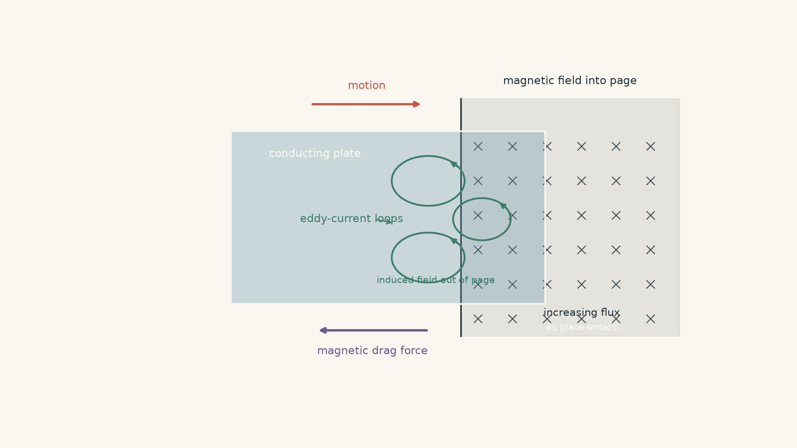
A useful mental model is to imagine many invisible wire loops drawn inside the plate. Some loops are entering the magnetic field while others may already be inside it. Changing flux drives current around those loops.
The model has a limit: the plate doesn’t really contain pre-drawn separate wires. Current can follow continuous paths through the metal. The imaginary loops simply help us picture why closed currents can exist.
The induced eddy currents produce their own magnetic fields. By Lenz’s law, their effect opposes the change that created them.
So:
- when a plate enters a magnetic field region, the magnetic force resists its entry,
- when it leaves, the induced current reverses, but the resulting force still resists its departure.
That is why eddy currents can create magnetic braking.
Cutting slots into the plate interrupts the large current paths. The eddy currents become smaller, so the braking effect and energy loss decrease. The same principle is important when studying Eddy-Current Losses in Transformers.
There is another useful boundary case. Suppose a conducting plate translates steadily while remaining completely inside a perfectly uniform magnetic field, with its orientation unchanged. In the idealised model, there is no continuing change of flux through loops fixed in the plate, so there is no sustained eddy-current braking purely from that translation.
Again, “metal moving through a field” is not enough by itself.
09A decision rule for moving-magnet questions
When you see motion and induction in an HSC problem, don’t immediately reach for \(B\ell v\).
Work through these questions instead.
1. Is there a complete loop or coil?
If yes, start by asking whether its magnetic flux is changing.
Check whether any of these are changing:
- \(B\), the magnetic field strength,
- \(A\), the area threaded by the field,
- \(\theta\), the angle between the field and area normal, or
- the position of the circuit in a non-uniform magnetic field.
2. Is it a straight conductor moving through a magnetic field?
For the standard perpendicular moving-rod arrangement, use
\[
\varepsilon=B\ell v
\]
and determine the direction of magnetic force on the charges.
3. Is the entire loop merely translating inside a uniform field?
If \(B\), \(A\), and \(\theta\) remain constant, the net emf is zero.
Do not award an emf just because everything is moving.
4. Is the conductor crossing a field boundary or moving through a non-uniform field?
Then the flux can change even if the loop’s area and orientation are fixed.
5. Does the problem ask for current direction?
First determine whether the original flux is increasing or decreasing. Then use Lenz’s law: the induced magnetic field opposes that change, not necessarily the original magnetic field itself.
10Questions and solutions
Question 1
A 200-turn coil experiences magnetic flux of \(2.5\times10^{-4}\text{ Wb}\) through each turn. A magnet is moved away, causing the flux to decrease uniformly to \(1.0\times10^{-4}\text{ Wb}\) in \(0.030\text{ s}\).
Calculate the magnitude of the average induced emf.
If the original magnetic flux is directed into the page, state the direction of the induced conventional current as viewed from the front of the page.
Solution 1
The average induced emf is \(1.0\text{ V}\), and the induced current is clockwise.
The flux through each turn decreases by
\[
\begin{aligned}
|\Delta\Phi|
&=|1.0\times10^{-4}-2.5\times10^{-4}|\\
&=1.5\times10^{-4}\text{ Wb}
\end{aligned}
\]
Faraday’s law gives
\[
\begin{aligned}
|\varepsilon|
&=N\frac{|\Delta\Phi|}{\Delta t}\\
&=200\left(\frac{1.5\times10^{-4}}{0.030}\right)\\
&=1.0\text{ V}
\end{aligned}
\]
For the direction, the flux into the page is decreasing. The induced current therefore creates a magnetic field into the page to oppose that decrease.
Using the right-hand grip rule, a clockwise conventional current produces a field into the page.
The tempting mistake is to say that the induced field must point opposite to the original field. Lenz’s law does not say that. It says the induced effect opposes the change. Because the original into-page flux is decreasing, the induced field points into the page as well.
Question 2
An 80-turn square coil has side length \(0.12\text{ m}\) and total resistance \(4.0\,\Omega\). It moves at \(2.0\text{ m s}^{-1}\) into a region containing a uniform \(0.50\text{ T}\) magnetic field directed into the page.
One edge of the coil remains parallel to the boundary of the magnetic-field region.
Calculate:
a. the induced emf while the coil is entering the field,
b. the induced current during entry,
c. how long the entry process lasts, and
d. the induced emf after the coil is completely inside the uniform field.
Solution 2
During entry, the induced emf is \(9.6\text{ V}\), the current is \(2.4\text{ A}\), and entry lasts \(0.060\text{ s}\). Once the coil is completely inside the uniform field, the induced emf is zero.
As the square enters, its overlap area with the magnetic field increases.
If its side length is \(L\), then
\[
\frac{\Delta A}{\Delta t}=Lv
\]
so the rate of flux change through one turn is
\[
\frac{\Delta\Phi}{\Delta t}=BLv
\]
The emf magnitude is therefore
\[
\begin{aligned}
|\varepsilon|
&=NBLv\\
&=(80)(0.50)(0.12)(2.0)\\
&=9.6\text{ V}
\end{aligned}
\]
The current is
\[
\begin{aligned}
I&=\frac{\varepsilon}{R}\\
&=\frac{9.6}{4.0}\\
&=2.4\text{ A}
\end{aligned}
\]
For the entire coil to enter, it must move one side length:
\[
\begin{aligned}
t&=\frac{L}{v}\\
&=\frac{0.12}{2.0}\\
&=0.060\text{ s}
\end{aligned}
\]
Once the coil is completely inside the field, it can keep moving while the flux stays constant:
\[
\Phi=BA=\text{constant}
\]
Therefore,
\[
\varepsilon=0
\]
The tempting route is to keep using \(NBLv\) after the coil is completely inside the field simply because it is still moving. That expression applied during entry because the field-threaded area was changing. Once the whole coil is inside a uniform field, the leading and trailing sides produce equal and opposite motional contributions, so the net emf is zero.
Question 3
A solid copper plate moves horizontally into, through, and then out of a small region containing a strong magnetic field perpendicular to the plate.
A second, otherwise identical plate contains several long slots that interrupt large current paths.
Explain:
a. why the solid plate experiences a force opposing its motion as it enters the field,
b. why the eddy-current direction reverses as the plate leaves the field even though the magnetic force still opposes the motion,
c. why the slotted plate experiences less braking, and
d. what would happen in the idealised case if the plate translated at constant velocity while remaining entirely inside a perfectly uniform magnetic field with fixed orientation.
Solution 3
The solid plate is braked because changing magnetic flux produces eddy currents whose magnetic effects oppose the plate’s motion; the eddy currents reverse on exit, the slots weaken the currents, and an ideal plate translating entirely inside a uniform field experiences no sustained eddy-current braking from that translation alone.
As the solid plate enters the field region, increasing portions of the metal become threaded by magnetic flux. This changing flux induces closed eddy-current paths within the conductor.
By Lenz’s law, the magnetic field produced by those currents acts to oppose the increase in flux. The interaction between the induced currents and the external magnetic field produces a force opposing the plate’s entry.
As the plate leaves, the situation changes. Flux through loops in the plate is now decreasing rather than increasing. The eddy currents therefore reverse so that their magnetic field tends to maintain the disappearing flux.
Although the current reverses, the force again opposes the plate’s motion. On entry, the plate is resisted from entering. On exit, it is resisted from leaving. In both cases mechanical energy is transferred into thermal energy in the plate.
The slotted plate experiences less braking because the slots interrupt large closed conducting paths. Smaller available loops generally have lower induced emfs and larger effective resistance for large-scale circulation, so the eddy currents are reduced.
In the final idealised case, a plate translating entirely inside a perfectly uniform static field has no ongoing change of magnetic flux through loops fixed within the plate, provided its orientation is unchanged. After any necessary charge redistribution, there is no sustained eddy-current braking caused simply by the uniform translation.
A tempting explanation is “the plate is moving through magnetic field lines, so eddy currents must always exist”. That picture fails here. Flux change, not motion alone, is the reliable test.
Question 4
A 40-turn rectangular coil is partly inside a magnetic-field region. The field is directed into the page.
The coil has height \(0.10\text{ m}\). Over a \(0.20\text{ s}\) interval:
- the width of the coil overlapping the magnetic field decreases linearly from \(0.080\text{ m}\) to \(0.040\text{ m}\), while
- the magnetic field strength increases linearly from \(0.40\text{ T}\) to \(0.70\text{ T}\).
The coil has resistance \(2.0\,\Omega\).
a. Calculate the magnitude of the average induced emf over the full \(0.20\text{ s}\).
b. Does the induced current maintain the same direction throughout the interval? Justify your answer quantitatively.
c. If the current reverses, determine the time after the beginning of the interval when the reversal occurs.
Solution 4
The average emf magnitude over the full interval is \(0.080\text{ V}\), but the current does not keep the same direction. It reverses \(0.0667\text{ s}\) after the interval begins.
The trap is to notice that \(B\) increases and immediately decide that flux must increase. The overlap area is decreasing at the same time, so the product \(BA\) must be examined.
Initially, the area inside the field is
\[
A_i=(0.10)(0.080)=0.0080\text{ m}^2
\]
so the initial flux per turn is
\[
\begin{aligned}
\Phi_i&=B_iA_i\\
&=(0.40)(0.0080)\\
&=0.0032\text{ Wb}
\end{aligned}
\]
Finally,
\[
A_f=(0.10)(0.040)=0.0040\text{ m}^2
\]
and
\[
\begin{aligned}
\Phi_f&=B_fA_f\\
&=(0.70)(0.0040)\\
&=0.0028\text{ Wb}
\end{aligned}
\]
The change in flux per turn over the complete interval is therefore
\[
\Delta\Phi=0.0028-0.0032=-4.0\times10^{-4}\text{ Wb}
\]
Hence,
\[
\begin{aligned}
|\varepsilon_{\text{avg}}|
&=N\frac{|\Delta\Phi|}{\Delta t}\\
&=40\left(\frac{4.0\times10^{-4}}{0.20}\right)\\
&=0.080\text{ V}
\end{aligned}
\]
That answers part a, but it does not prove that the current had one constant direction for the whole interval.
Let \(t\) be the time in seconds after the interval begins.
The field increases at
\[
\frac{\Delta B}{\Delta t}
=\frac{0.70-0.40}{0.20}
=1.5\text{ T s}^{-1}
\]
so
\[
B=0.40+1.5t
\]
The overlap width falls at
\[
\frac{0.040-0.080}{0.20}
=-0.20\text{ m s}^{-1}
\]
so
\[
w=0.080-0.20t
\]
The overlap area is
\[
A=0.10w=0.0080-0.020t
\]
The flux through one turn is
\[
\Phi=BA
\]
For a small change in time, the rate of change is
\[
\frac{d\Phi}{dt}
=A\frac{dB}{dt}+B\frac{dA}{dt}
\]
Substituting the expressions above,
\[
\begin{aligned}
\frac{d\Phi}{dt}
&=(0.0080-0.020t)(1.5)+(0.40+1.5t)(-0.020)\\
&=0.0040-0.060t
\end{aligned}
\]
The current reverses when the instantaneous flux stops increasing and starts decreasing, so set
\[
\frac{d\Phi}{dt}=0
\]
giving
\[
\begin{aligned}
0.0040-0.060t&=0\\
t&=\frac{0.0040}{0.060}\\
&=0.0667\text{ s}
\end{aligned}
\]
Before \(0.0667\text{ s}\), the into-page flux is increasing, so the induced field points out of the page.
After \(0.0667\text{ s}\), the into-page flux is decreasing, so the induced field points into the page.
The current therefore reverses.
The surprising part is that the average flux over the entire interval decreases even though it initially increases. An average emf calculation alone can hide a change of direction inside the interval.
Question 5
A single-turn square conducting loop has side length \(0.20\text{ m}\), resistance \(0.30\,\Omega\), and moves to the right at \(3.0\text{ m s}^{-1}\).
It remains completely inside a magnetic field directed into the page, but the field is not uniform. Its magnitude varies with horizontal position \(x\) according to
\[
B(x)=0.40+(0.50)x
\]
where \(B\) is in teslas and \(x\) is in metres.
At one instant, the left edge of the loop is at \(x=0.60\text{ m}\).
a. Calculate the motional emf produced along each vertical side of the loop.
b. Hence determine the net emf around the loop and the current.
c. State the current direction.
d. A student argues that because the loop is completely inside the magnetic field and its area and orientation are constant, its emf must be zero. Explain exactly why that argument fails.
e. Another student replaces the non-uniform field with a uniform \(0.75\text{ T}\) field. The loop continues moving at the same speed. Determine the net emf now, and explain why using \(B\ell v\) on only one side would give the wrong conclusion.
Solution 5
In the non-uniform field, the loop has a net emf of \(0.060\text{ V}\) and an anticlockwise current of \(0.20\text{ A}\). In the uniform \(0.75\text{ T}\) field, the net emf is zero.
This problem exposes the limit of the shortcut “a loop completely inside a field has no emf”. That statement is only safe when the magnetic flux remains constant. Here the loop moves into progressively stronger magnetic field.
The left vertical side is at
\[
x_L=0.60\text{ m}
\]
so its field strength is
\[
\begin{aligned}
B_L&=0.40+(0.50)(0.60)\\
&=0.70\text{ T}
\end{aligned}
\]
The right edge is \(0.20\text{ m}\) further right:
\[
x_R=0.80\text{ m}
\]
so
\[
\begin{aligned}
B_R&=0.40+(0.50)(0.80)\\
&=0.80\text{ T}
\end{aligned}
\]
For the left side,
\[
\begin{aligned}
\varepsilon_L
&=B_L\ell v\\
&=(0.70)(0.20)(3.0)\\
&=0.42\text{ V}
\end{aligned}
\]
For the right side,
\[
\begin{aligned}
\varepsilon_R
&=B_R\ell v\\
&=(0.80)(0.20)(3.0)\\
&=0.48\text{ V}
\end{aligned}
\]
The two vertical sides drive current in opposite senses around the loop. Because they experience different magnetic field strengths, they do not cancel.
The net emf magnitude is
\[
\begin{aligned}
|\varepsilon_{\text{net}}|
&=|\varepsilon_R-\varepsilon_L|\\
&=0.48-0.42\\
&=0.060\text{ V}
\end{aligned}
\]
The current is therefore
\[
\begin{aligned}
I&=\frac{\varepsilon_{\text{net}}}{R}\\
&=\frac{0.060}{0.30}\\
&=0.20\text{ A}
\end{aligned}
\]
As the loop moves right, it enters regions with larger \(B\). Its into-page magnetic flux therefore increases.
Lenz’s law requires the induced current to create a field out of the page. Using the right-hand grip rule, that requires an anticlockwise conventional current.
For part d, the student’s argument correctly notes that \(A\) and \(\theta\) are constant but incorrectly treats \(B\) as constant.
The loop moves through a field gradient, so the magnetic field threading it becomes stronger with time. Its flux therefore changes even though the loop is always completely inside the magnetic-field region.
Another way to check the result is to consider the field at the centre of the loop. The centre moves through a field gradient of
\[
0.50\text{ T m}^{-1}
\]
at \(3.0\text{ m s}^{-1}\), so its representative field increases at
\[
\begin{aligned}
\frac{dB}{dt}
&=(0.50)(3.0)\\
&=1.5\text{ T s}^{-1}
\end{aligned}
\]
The square has area
\[
A=(0.20)^2=0.040\text{ m}^2
\]
so
\[
\begin{aligned}
|\varepsilon|
&=A\frac{dB}{dt}\\
&=(0.040)(1.5)\\
&=0.060\text{ V}
\end{aligned}
\]
which agrees with the motional-emf calculation.
For part e, in a uniform \(0.75\text{ T}\) field, each vertical side has motional emf magnitude
\[
\begin{aligned}
\varepsilon_{\text{side}}
&=B\ell v\\
&=(0.75)(0.20)(3.0)\\
&=0.45\text{ V}
\end{aligned}
\]
But the two sides act in opposite senses around the loop, so
\[
\varepsilon_{\text{net}}=0.45-0.45=0
\]
and no current flows.
The tempting mistake is to calculate \(B\ell v=0.45\text{ V}\) for one side and stop. That gives the emf associated with that individual conductor, not the net emf around the complete loop.
The deeper rule survives every version of the problem: inspect the whole circuit and ask whether its magnetic flux linkage is changing.
11What this idea lets you do next
Once you can decide whether motion actually changes magnetic flux, induction questions become much more systematic.
For a coil, identify what changes in \(B\), \(A\), or \(\theta\), then use Faraday’s law for the emf. For a moving straight conductor, \(B\ell v\) can give the motional emf in the standard geometry. For a closed loop, always check whether different motional emfs cancel. For a metal plate, think about changing flux through possible current paths and the resulting eddy currents.
The next step is direction. Once the flux change is known, Lenz’s law tells you which way the induced current must act. That same reasoning then carries directly into generators, electromagnetic braking, and transformers.