
Current as Charge Flow Rate: Using I = q/t in HSC Physics
Learn how electric current measures the rate of charge flow, how to use I = q/t for steady current, and how to avoid common calculation mistakes.
A wire carries 12 C of charge past a point in 3.0 s. Another wire carries 15 C past a point in 5.0 s. Which wire has the larger current?
It is tempting to choose the second wire because 15 C is more charge. But current does not tell you how much charge passes. It tells you how quickly charge passes. Once time is included, the first wire actually has the larger current.
That idea is the whole purpose of \(I = q/t\).
01Current measures a rate, not an amount
Picture one fixed point in a wire. We are going to count how much electric charge crosses that point.
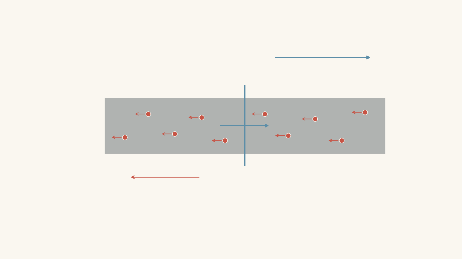
Suppose 20 C crosses the point.
That information alone is not enough to tell us the current. Did the 20 C cross in 1 second, 10 seconds, or an hour?
Now suppose 20 C crosses in 4 seconds. We can say that, on average, 5 C crosses each second.
That rate of charge flow is the electric current.
For steady current,
\[
I = \frac{q}{t}
\]
where:
- \(I\) is current, measured in amperes (A)
- \(q\) is charge that passes a point, measured in coulombs (C)
- \(t\) is the time interval, measured in seconds (s)
So:
\[
1\text{ A} = 1\text{ C s}^{-1}
\]
A current of 1 A means 1 C of charge passes a point every second.
Before going further, predict this: if twice as much charge passes a point in twice as much time, what happens to the current?
It stays the same. Both the numerator and denominator in \(I = q/t\) double, so their ratio does not change.
For example,
\[
\frac{4\text{ C}}{2\text{ s}} = 2\text{ A}
\]
and
\[
\frac{8\text{ C}}{4\text{ s}} = 2\text{ A}
\]
More charge has flowed in the second case, but it has also had proportionally more time to do so.
02What “steady charge flow” means
The equation \(I = q/t\) is especially simple when the current is steady.
A steady current means the rate of charge flow stays constant with time. If the current is 3 A, then 3 C passes a point each second:
- after 1 s, 3 C has passed
- after 2 s, 6 C has passed
- after 5 s, 15 C has passed
The charge accumulated over time follows
\[
q = It
\]
This is just the same equation rearranged.
For steady current, a graph of charge \(q\) against time \(t\) would be a straight line. Its gradient is the current:
\[
I = \frac{\Delta q}{\Delta t}
\]
A steeper charge-time graph means charge is passing more quickly, so the current is larger.
The simple picture is slightly incomplete. In a real circuit, currents can change with time. In that case, dividing total charge by total time gives an average current over that interval, not necessarily the current at every instant. For this guide, we are mainly dealing with steady current, where those two ideas coincide.
03A useful way to picture current
Imagine students walking through a classroom doorway. The number of students who pass through is like the amount of charge \(q\). The time you watch the doorway is \(t\). The number passing per second is like current \(I\).
If 30 students leave in 10 s, the flow rate is 3 students per second. If another doorway has 20 students leave in 4 s, the second doorway has the greater flow rate even though fewer students passed in total.
The analogy has a limit. Electric charge is not literally a queue of students, and in a metal the mobile charge carriers are electrons distributed throughout the conductor. If you need to revise what is actually moving in a metal, see Electric Current in Metals: Charge Carriers and Drift.
The doorway idea is useful for one thing: current depends on charge per unit time.
04Worked example: Finding current from charge and time
A steady flow transfers 24 C of charge through a point in a wire during 6.0 s. Calculate the current.
Step 1
The charge is \(q = 24\text{ C}\), and the time is \(t = 6.0\text{ s}\).
We need the current \(I\).
Step 2
\[
I = \frac{q}{t}
\]
Step 3
\[
I = \frac{24\text{ C}}{6.0\text{ s}} = 4.0\text{ C s}^{-1}
\]
Since \(1\text{ C s}^{-1} = 1\text{ A}\),
\[
I = 4.0\text{ A}
\]
Step 4
A current of 4.0 A means 4.0 C of charge passes that point every second.
05Rearranging \(I = q/t\)
You should be able to find any one of \(I\), \(q\), or \(t\) if the other two are known.
Starting from
\[
I = \frac{q}{t}
\]
multiply both sides by \(t\):
\[
q = It
\]
Then, if time is unknown:
\[
t = \frac{q}{I}
\]
A compact decision table is useful:
| You need | Use |
|---|---|
| Current | \(I = \frac{q}{t}\) |
| Charge | \(q = It\) |
| Time | \(t = \frac{q}{I}\) |
Do not memorise these as three unrelated formulas. They are all the same relationship: current measures how rapidly charge is transferred.
06Watch the time units
The SI unit of time in \(I = q/t\) is the second.
So if a question gives 2.5 minutes, convert it before substituting:
\[
2.5\text{ min} = 2.5 \times 60 = 150\text{ s}
\]
This is an easy place to lose a factor of 60.
Similarly:
\[
1\text{ ms} = 1\times10^{-3}\text{ s}
\]
and
\[
1\text{ \(\mu\)s} = 1\times10^{-6}\text{ s}
\]
The current equation itself has not changed. Only the unit conversion has.
07Worked example: From current to number of electrons
A steady current of 0.80 A flows through a metal wire for 2.5 minutes. Calculate the number of electrons that pass a point in the wire during this time. Use the magnitude of the electron charge \(e = 1.60\times10^{-19}\text{ C}\).
This problem adds one extra step. First find the total charge using \(q = It\). Then connect total charge to the number of electrons.
Step 1
\[
t = 2.5\times60 = 150\text{ s}
\]
Step 2
Using
\[
q = It
\]
we get
\[
q = (0.80\text{ A})(150\text{ s}) = 120\text{ C}
\]
Remember that an ampere is a coulomb per second, so the seconds cancel appropriately.
Step 3
If \(N\) electrons pass the point, the magnitude of the total charge is
\[
q = Ne
\]
where \(e = 1.60\times10^{-19}\text{ C}\).
Rearranging,
\[
N = \frac{q}{e}
\]
Step 4
\[
N = \frac{120\text{ C}}{1.60\times10^{-19}\text{ C}}
= 7.5\times10^{20}
\]
So,
\[
N = 7.5\times10^{20}\text{ electrons}
\]
A current that looks quite ordinary on a circuit diagram corresponds to an enormous number of electrons passing a cross-section of the wire.
Notice that we used the magnitude of the electron charge here. An electron itself has charge \(-1.60\times10^{-19}\text{ C}\), but the negative sign describes the type of charge and its relationship to the conventional current direction. It does not mean there is a “negative number” of electrons.
08The main misconception: more charge means more current
Return to the opening comparison.
Wire A transfers 12 C in 3.0 s:
\[
I_A = \frac{12}{3.0} = 4.0\text{ A}
\]
Wire B transfers 15 C in 5.0 s:
\[
I_B = \frac{15}{5.0} = 3.0\text{ A}
\]
Wire A has the larger current even though less total charge passed.
Why does the wrong prediction feel reasonable? Because everyday language encourages us to think “more stuff moving” must mean “more flow”. But flow rate always involves time.
The same distinction appears with water. Filling a 10 L bucket does not tell you the flow rate of the tap unless you also know how long the filling took.
So when comparing currents, never compare \(q\) alone. Compare the ratio \(q/t\).
09Current and electron motion are related, but not identical ideas
In a metal, electrons are the mobile charge carriers. Their motion produces an electric current.
But current is not “the speed of the electrons”. It is a rate of charge transfer.
Two situations could have the same current even if the microscopic behaviour of the charge carriers differs, provided the same amount of charge crosses a chosen cross-section each second.
That is why \(I = q/t\) is so useful. It lets us describe charge flow at the circuit level without having to track individual electrons.
10Questions and solutions
Question 1
A steady current transfers 18 C of charge through a point in 6.0 s. Calculate the current.
Solution 1
The current is 3.0 A because current is charge transferred per unit time.
Using
\[
I = \frac{q}{t}
\]
with \(q = 18\text{ C}\) and \(t = 6.0\text{ s}\),
\[
I = \frac{18\text{ C}}{6.0\text{ s}}
= 3.0\text{ C s}^{-1}
= 3.0\text{ A}
\]
So 3.0 C of charge passes the point each second.
Question 2
Two wires carry steady currents.
In wire P, 24 C passes a point in 3.0 s. In wire Q, 30 C passes a point in 5.0 s.
Which wire has the larger current? Explain why comparing the total charge alone gives the wrong conclusion.
Solution 2
Wire P has the larger current, 8.0 A compared with 6.0 A in wire Q. The total charge alone cannot determine current because current depends on both charge and time.
For wire P,
\[
I_P = \frac{24\text{ C}}{3.0\text{ s}}
= 8.0\text{ A}
\]
For wire Q,
\[
I_Q = \frac{30\text{ C}}{5.0\text{ s}}
= 6.0\text{ A}
\]
Wire Q transfers more total charge, but it takes longer to do so. Wire P transfers charge at the greater rate.
The tempting mistake is to see \(30\text{ C} > 24\text{ C}\) and conclude that wire Q must have the greater current. That ignores the denominator in \(I = q/t\).
Question 3
A device draws a steady current of 0.40 A for 2.5 minutes. Calculate the total charge that passes through the device.
Solution 3
The total charge transferred is 60 C.
First convert the time to seconds:
\[
t = 2.5\times60 = 150\text{ s}
\]
For steady current,
\[
q = It
\]
so
\[
q = (0.40\text{ A})(150\text{ s})
= 60\text{ C}
\]
Therefore, 60 C of charge passes through the device during the 2.5 minute interval.
A common mistake is to substitute \(2.5\) directly as the time. The ampere is defined using seconds, so the time must first be expressed in seconds.
Question 4
A steady current of 3.2 mA flows through a conductor for 40 s. Calculate:
(a) the charge transferred, and
(b) the number of electrons corresponding to this amount of charge.
Use \(e = 1.60\times10^{-19}\text{ C}\).
Solution 4
The charge transferred is \(0.128\text{ C}\), corresponding to \(8.0\times10^{17}\) electrons.
For part (a), first convert the current:
\[
3.2\text{ mA} = 3.2\times10^{-3}\text{ A}
\]
Using
\[
q = It
\]
gives
\[
q = (3.2\times10^{-3}\text{ A})(40\text{ s})
= 0.128\text{ C}
\]
For part (b),
\[
q = Ne
\]
so
\[
N = \frac{q}{e}
\]
Substituting,
\[
N = \frac{0.128\text{ C}}{1.60\times10^{-19}\text{ C}}
= 8.0\times10^{17}
\]
Therefore,
\[
N = 8.0\times10^{17}\text{ electrons}
\]
The very large number is reasonable. One electron carries an extremely small amount of charge, so even modest currents involve huge numbers of charge carriers.
Question 5
A student measures charge passing a point in a circuit.
During the first 3.0 s, 6.0 C passes the point. During the next 2.0 s, another 8.0 C passes.
The student calculates
\[
I = \frac{14\text{ C}}{5.0\text{ s}} = 2.8\text{ A}
\]
and claims that the current was a steady 2.8 A throughout the full 5.0 s.
Is that conclusion justified? Calculate the current during each interval and explain what the value 2.8 A actually represents.
Solution 5
No. The current was not steady at 2.8 A. The value 2.8 A is the average current over the full 5.0 s.
During the first interval,
\[
I_1 = \frac{q_1}{t_1}
= \frac{6.0\text{ C}}{3.0\text{ s}}
= 2.0\text{ A}
\]
During the second interval,
\[
I_2 = \frac{q_2}{t_2}
= \frac{8.0\text{ C}}{2.0\text{ s}}
= 4.0\text{ A}
\]
The current therefore changed from 2.0 A to 4.0 A.
Across the complete interval, the total charge is
\[
q_{\text{total}} = 6.0 + 8.0 = 14.0\text{ C}
\]
and the total time is
\[
t_{\text{total}} = 3.0 + 2.0 = 5.0\text{ s}
\]
so the average current is
\[
I_{\text{avg}}
= \frac{q_{\text{total}}}{t_{\text{total}}}
= \frac{14.0\text{ C}}{5.0\text{ s}}
= 2.8\text{ A}
\]
The trap is assuming that one value of \(q/t\) over a long interval proves the current had that value at every moment. It does not. For a genuinely steady current, equal time intervals would transfer charge at the same rate.
11What this idea lets you do next
Once current is understood as charge flow rate, several later electricity ideas become easier to interpret.
You can connect the circuit-level quantity \(I\) to the microscopic motion of charge carriers in a metal, rather than thinking of current as a mysterious substance travelling through a wire. You can also interpret charge-time graphs, distinguish steady from changing current, and calculate how much charge passes through circuit components over a known time.
The key decision is simple: whenever you see a current problem, ask “How much charge passes, and how long does it take?” If those two quantities are connected by a constant rate, \(I = q/t\) describes the flow directly.