
Magnetic Field Models: From Field Lines to Field Strength
Learn how magnetic field-line diagrams show direction and relative strength, then connect them to measured and calculated values of magnetic field strength.
Two students sketch the magnetic field around the same bar magnet. One draws eight field lines. The other draws twenty. Has the second student accidentally created a stronger magnet?
No. The number of lines on the page is partly a drawing choice. But the way those lines are arranged still tells us something important about the real field.
That is the problem magnetic field models have to solve. A field-line diagram is excellent for showing direction, shape, and relative strength. It does not automatically tell you that the field is \(3.2 \times 10^{-3}\ \text{T}\). For that, you need a measurement or a calculation.
The useful skill is moving between those two descriptions without treating either one as more physical than it really is.
01What a field-line diagram is actually telling you
Imagine placing a tiny compass at different points around a magnet. At each position, the compass settles in a particular direction.
Now imagine drawing a short arrow wherever you put the compass. If you join arrows that point smoothly into one another, you get magnetic field lines.
The lines are therefore a model of a vector field. At every point where the magnetic field is non-zero, the field has:
- a direction, and
- a magnitude, or strength.
The magnetic field vector is written as \(\vec B\). Its magnitude is written as \(B\).
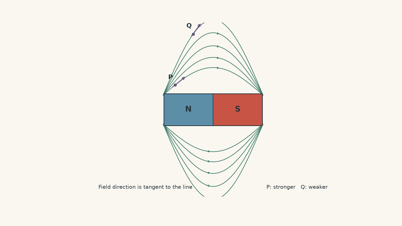
Direction comes from the tangent
Suppose you choose a point on one curved field line. Which way does the magnetic field point there?
Do not point towards the nearest magnet pole. Instead, imagine a tiny arrow touching the curve at that exact point. The magnetic field points along that tangent.
For a permanent magnet, field-line arrows point from the north pole towards the south pole outside the magnet.
Around a current-carrying straight wire, the lines form circles. Their direction comes from the right-hand grip rule. You can review that geometry in Magnetic Field Around a Current-Carrying Wire: HSC Physics.
Line spacing represents relative field strength
Now compare point P close to a magnet pole with point Q farther away.
Before reading on, predict what a magnetic-field sensor would usually show. Would \(B\) be larger at P or Q?
P. In a consistent field-line diagram, crowded lines represent a stronger field, while widely separated lines represent a weaker field.
This gives us a qualitative model:
| Field-line feature | Physical interpretation |
|---|---|
| Lines close together | Relatively large \(B\) |
| Lines far apart | Relatively small \(B\) |
| Straight, parallel, similarly spaced lines | Approximately uniform field |
| Curved lines | Field direction changes with position |
| Arrow on a line | Direction of \(\vec B\) |
| No field lines crossing at an ordinary point | Only one field direction exists at that point |
The word relative matters.
If P has visibly denser lines than Q, you can reasonably conclude that \(B_P>B_Q\). You generally cannot conclude that \(B_P=3B_Q\) just because the drawing seems to contain three times as many lines per centimetre.
02The field lines are not magnetic spaghetti
A tempting picture is that a magnet somehow fires invisible strands through space, and a stronger magnet contains more strands.
It does not.
Field lines are invented lines that help us represent a field that exists continuously throughout space. You could add another five lines to your sketch without changing the magnet at all.
A useful analogy is a contour map of a mountain. Crowded contour lines tell you the terrain is changing rapidly, just as crowded field lines indicate a strong magnetic field in the usual drawing convention.
The analogy breaks in one important place. Real topographic contour lines normally have labelled heights, such as 200 m or 250 m. An ordinary HSC magnetic field-line sketch does not come with a numerical value attached to each line.
Unless a diagram has been specifically calibrated, line density is qualitative rather than numerical.
That distinction prevents one of the most common mistakes in this topic:
More lines drawn does not necessarily mean a larger magnetic field. Closer lines within a consistently drawn field map indicate a larger magnetic field.
03Turning the picture into a number
For a quantitative magnetic field model, we want an actual value of \(B\).
In HSC Physics, \(B\) is normally measured in tesla, symbol \(\text{T}\). More precisely, \(B\) is magnetic flux density, although HSC questions will often discuss it simply as magnetic field strength.
Useful smaller units are:
\[ 1\ \text{mT}=10^{-3}\ \text{T} \]
and
\[ 1\ \mu\text{T}=10^{-6}\ \text{T}. \]
There are two main ways to obtain a numerical field value:
- measure it, or
- calculate it from a model.
Measuring \(B\)
A Hall probe can measure magnetic field at a particular position.
Suppose you move a Hall probe away from one pole of a magnet. A field-line sketch predicts that the field should weaken as the lines spread out. The Hall probe turns that qualitative prediction into numbers.
You might obtain data such as:
| Position | Measured \(B\) |
|---|---|
| Close to pole | \(4.8\ \text{mT}\) |
| Further away | \(2.1\ \text{mT}\) |
| Much further away | \(0.7\ \text{mT}\) |
The diagram and the measurement are describing the same field at different levels of detail.
There is one experimental detail worth remembering. A Hall sensor can be sensitive to the component of the magnetic field along a particular axis. Orientation therefore matters. A strangely small reading does not necessarily mean the field itself is weak; the probe may simply be badly aligned.
04Calculating the field around a long straight wire
Some field shapes have simple mathematical models.
For a long, straight wire carrying current \(I\), the magnetic field a perpendicular distance \(r\) from the wire is
\[ B=\frac{\mu_0 I}{2\pi r}, \]
where:
- \(B\) is magnetic field strength in tesla, \(\text{T}\),
- \(I\) is current in amperes, \(\text{A}\),
- \(r\) is perpendicular distance from the wire in metres, \(\text{m}\), and
- \(\mu_0=4\pi\times10^{-7}\ \text{T m A}^{-1}\) is the permeability of free space.
Look at what the equation says before doing any arithmetic.
For a fixed current,
\[ B\propto\frac{1}{r}. \]
So if you double your distance from the wire, predict what happens to \(B\).
It halves.
That should also affect your qualitative sketch. Circular field lines drawn near the wire should represent a stronger field than regions farther from the wire.
Worked example: Field strength beside a straight wire
A long straight wire carries a current of \(6.0\ \text{A}\). Calculate the magnetic field strength \(4.0\ \text{cm}\) from the wire. Then predict the field strength at \(8.0\ \text{cm}\).
Step 1
\[ r=4.0\ \text{cm}=0.040\ \text{m}. \]
Step 2
\[ \begin{aligned} B&=\frac{\mu_0 I}{2\pi r}\\ &=\frac{(4\pi\times10^{-7})(6.0)} {2\pi(0.040)}\\ &=3.0\times10^{-5}\ \text{T}. \end{aligned} \]
So the field is
\[ B=30\ \mu\text{T}. \]
Step 3
At \(8.0\ \text{cm}\), \(r\) has doubled. Because \(B\propto 1/r\),
\[ B=\frac{30\ \mu\text{T}}{2}=15\ \mu\text{T}. \]
The result matches the field-line model: as you move away from the wire, the field becomes weaker. The numerical calculation tells us exactly how much weaker for an ideal long straight wire.
05Calculating the field inside a solenoid
A long solenoid produces another particularly useful field pattern.
Near the centre, the field lines are approximately straight, parallel, and evenly spaced. That is the visual signature of an approximately uniform magnetic field.
For an ideal long solenoid in air,
\[ B=\mu_0 nI, \]
where \(n\) is the number of turns per metre.
Since
\[ n=\frac{N}{L}, \]
we can also write
\[ B=\mu_0\frac{N}{L}I, \]
where:
- \(N\) is the total number of turns,
- \(L\) is the solenoid length in metres, and
- \(I\) is the current in amperes.
The model predicts something the field-line drawing only hints at. Increasing the current increases \(B\). Increasing the number of turns per metre also increases \(B\).
The details of the field pattern are covered in Magnetic Field Inside a Solenoid: HSC Physics Explained.
There is an important limitation. The equation assumes a long ideal solenoid and works best near its centre. A real solenoid has ends, so its field becomes less uniform near those ends.
Worked example: Comparing a solenoid model with a measurement
A solenoid has \(1200\) turns, a length of \(0.60\ \text{m}\), and carries a current of \(1.8\ \text{A}\). Calculate the ideal magnetic field near its centre. A Hall probe measures \(4.25\ \text{mT}\). Compare the measurement with the model.
Step 1
\[ n=\frac{N}{L} =\frac{1200}{0.60} =2000\ \text{m}^{-1}. \]
Step 2
\[ \begin{aligned} B&=\mu_0 nI\\ &=(4\pi\times10^{-7})(2000)(1.8)\\ &=4.52\times10^{-3}\ \text{T}. \end{aligned} \]
Therefore,
\[ B_{\text{ideal}}=4.52\ \text{mT}. \]
Step 3
The Hall probe gives
\[ B_{\text{measured}}=4.25\ \text{mT}. \]
The difference is
\[ 4.52-4.25=0.27\ \text{mT}. \]
Relative to the ideal prediction, this is approximately
\[ \frac{0.27}{4.52}\times100\%\approx6.0\%. \]
The measured field is about \(6\%\) lower than the ideal value.
That does not automatically mean the experiment is wrong. The equation assumes an ideal, sufficiently long solenoid and a measurement well away from the ends. A real coil has finite length, imperfect geometry, and measurement uncertainty.
The field-line model, equation, and measurement should agree in their broad prediction while still allowing sensible differences caused by the assumptions behind the equation.
06When the field comes from more than one source
Real magnetic fields often overlap.
Suppose two sources produce magnetic fields \(\vec B_1\) and \(\vec B_2\) at the same point. The actual field is not whichever one happens to look stronger in the diagram.
It is the vector sum:
\[ \vec B_{\text{net}}=\vec B_1+\vec B_2. \]
Direction now matters just as much as magnitude.
If two \(3\ \text{mT}\) fields point in the same direction, the net field is \(6\ \text{mT}\).
If they point in opposite directions, the net field is zero.
That zero is real even though both sources are still producing magnetic fields individually. The fields have not disappeared; their vectors cancel at that location.
This is where quantitative calculations can reveal something that is easy to miss in a sketch.
07How to decide which model to use
A useful HSC decision rule is:
| What the question asks | Best starting point |
|---|---|
| Which way does the field point? | Field-line tangent, compass direction, or right-hand rule |
| Where is the field relatively stronger? | Compare field-line spacing within the same consistent diagram |
| What is the numerical value of \(B\)? | Use an appropriate equation or measurement |
| What happens when distance or current changes? | Use proportional relationships from the equation |
| Several magnetic fields act together | Add the fields as vectors |
| Calculation and experiment differ slightly | Check the assumptions and uncertainty |
| Two separate sketches contain different numbers of lines | Do not compare line counts unless the representation is calibrated |
The key is not choosing between a qualitative and quantitative model. You usually need both.
The sketch tells you what sort of answer is physically sensible. The equation or measurement tells you how large the field actually is.
08The most tempting misconception
Suppose one diagram of a solenoid contains six internal field lines and another contains twelve.
Can you conclude the second solenoid has twice the magnetic field strength?
No.
The illustrator may simply have drawn more lines.
Now change the situation. Suppose both solenoids appear in the same carefully constructed diagram, using the same scale and the same line-density convention, and the lines inside one solenoid are clearly more crowded.
Then it is reasonable to infer that its field is stronger.
There is a deeper version of this idea. Field-line density can be made quantitative if the diagram is explicitly constructed so that every line represents the same amount of magnetic flux and the spatial scale is known. Ordinary HSC field sketches usually do not provide that calibration.
So do not measure the number of millimetres between two hand-drawn field lines and turn it into tesla. That is giving the sketch precision it never claimed to have.
09Questions and solutions
Question 1
A magnetic field-line diagram around a permanent magnet shows point P close to one pole, where the lines are crowded, and point Q farther away, where the lines are more widely separated. At P, the tangent to the field line points towards the right.
State the direction of the magnetic field at P and compare the field strength at P with the field strength at Q. Can the diagram alone be used to calculate the numerical ratio \(B_P/B_Q\)?
Solution 1
The magnetic field at P points to the right, and \(B_P>B_Q\), but the numerical ratio \(B_P/B_Q\) cannot normally be determined from an uncalibrated field-line sketch.
The field direction is tangent to the field line at P, so the right-pointing tangent gives the direction of \(\vec B\).
The lines are more crowded at P than at Q. Under the usual consistent drawing convention, this represents a stronger field at P.
The tempting mistake is to count lines or measure their page spacing and convert that directly into a ratio of field strengths. An ordinary field-line drawing gives relative strength, not a numerical scale. Without extra calibration, we cannot say that P is twice, three times, or any other exact multiple as strong as Q.
Question 2
A long straight vertical wire passes upwards through a horizontal bench. A Hall probe is aligned north-south and placed \(4.0\ \text{cm}\) east of the wire and then \(4.0\ \text{cm}\) west of it. Positive readings mean the field points north.
The measurements are:
- east of the wire: \(+55\ \mu\text{T}\),
- west of the wire: \(-5\ \mu\text{T}\).
Assume there is also a uniform background magnetic field directed north or south. Treat the wire as infinitely long.
Determine:
- the magnitude and direction of the background field,
- the magnetic field produced by the wire at \(4.0\ \text{cm}\),
- the current in the wire, and
- whether the current travels upwards or downwards through the bench.
Solution 2
The background field is \(25\ \mu\text{T}\) north, the wire produces \(30\ \mu\text{T}\) at \(4.0\ \text{cm}\), the current is \(6.0\ \text{A}\), and it travels upwards through the bench.
At equal distances on opposite sides of a straight wire, the wire’s magnetic field has the same magnitude but opposite directions.
Let \(B_0\) be the signed background field and \(B_w\) the wire’s field on the eastern side. Taking north as positive,
\[ B_0+B_w=55\ \mu\text{T} \]
and
\[ B_0-B_w=-5\ \mu\text{T}. \]
Adding the equations gives
\[ 2B_0=50\ \mu\text{T}, \]
so
\[ B_0=25\ \mu\text{T}. \]
The positive sign means north.
Substituting into the eastern measurement,
\[ 25+B_w=55, \]
so
\[ B_w=30\ \mu\text{T} =3.0\times10^{-5}\ \text{T}. \]
Now use
\[ B=\frac{\mu_0 I}{2\pi r}. \]
Rearranging,
\[ I=\frac{2\pi rB}{\mu_0}. \]
With \(r=0.040\ \text{m}\),
\[ \begin{aligned} I&=\frac{2\pi(0.040)(3.0\times10^{-5})} {4\pi\times10^{-7}}\\ &=6.0\ \text{A}. \end{aligned} \]
On the eastern side, the wire’s field points north. The right-hand grip rule therefore gives an upward current through the bench.
The tempting route is to substitute either Hall-probe reading directly into the straight-wire equation. That would incorrectly treat the total measured field as though it came only from the wire. The background field must first be separated from the wire’s contribution.
Question 3
Two long solenoids overlap along the same axis. Ignore end effects.
Solenoid A has \(1000\) turns per metre and carries \(2.0\ \text{A}\). Its field through the overlap points east.
Solenoid B has \(1500\) turns per metre and carries a current in the opposite sense, so its field points west.
A Hall probe in the overlap measures a net field of \(0.25\ \text{mT}\) east.
Calculate the current in solenoid B. Then compare the expected field-line density in the overlap with a region that is inside solenoid A but not solenoid B.
Solution 3
Solenoid B carries approximately \(1.20\ \text{A}\), and the field lines in the overlap should be much less dense than in a region containing only the field from solenoid A.
For an ideal solenoid,
\[ B=\mu_0 nI. \]
Solenoid A produces
\[ \begin{aligned} B_A &=(4\pi\times10^{-7})(1000)(2.0)\\ &=2.51\times10^{-3}\ \text{T}\\ &=2.51\ \text{mT}. \end{aligned} \]
Take east as positive. Because solenoid B produces a westward field,
\[ B_{\text{net}}=B_A-B_B. \]
Therefore,
\[ 0.25\times10^{-3} =\mu_0(1000)(2.0)-\mu_0(1500)I_B. \]
Divide by \(\mu_0\):
\[ \frac{0.25\times10^{-3}}{4\pi\times10^{-7}} =2000-1500I_B. \]
The left-hand side is approximately \(199\ \text{A m}^{-1}\), so
\[ 1500I_B\approx2000-199=1801. \]
Hence
\[ I_B\approx1.20\ \text{A}. \]
Inside solenoid A alone, the field is about \(2.51\ \text{mT}\). In the overlap, the net field is only \(0.25\ \text{mT}\), so a consistent qualitative field map should show far lower field-line density there.
The tempting error is to add \(B_A\) and \(B_B\) simply because there are two magnetic sources. Magnetic fields are vectors. Here their directions oppose, so the second solenoid reduces the net field instead of increasing it.
Question 4
Two long parallel wires pass perpendicularly out of a page. Their separation is \(12\ \text{cm}\).
The left wire carries \(6.0\ \text{A}\) out of the page. The right wire carries \(3.0\ \text{A}\) out of the page.
A student argues that the net magnetic field must be zero at the midpoint because the midpoint is equally far from both wires.
Find:
- the location between the wires where the net field is actually zero,
- the magnitude and direction of the net field at the midpoint, and
- how a good qualitative field-line representation should reflect the zero-field location.
Solution 4
The net field is zero \(8.0\ \text{cm}\) from the \(6.0\ \text{A}\) wire and \(4.0\ \text{cm}\) from the \(3.0\ \text{A}\) wire. At the midpoint, the net field is \(10\ \mu\text{T}\) upwards on the page.
Between two currents directed out of the page, the magnetic fields oppose one another.
Let \(x\) be the distance from the \(6.0\ \text{A}\) wire to the zero-field point. The distance from the \(3.0\ \text{A}\) wire is \(0.12-x\).
For cancellation, the field magnitudes must be equal:
\[ \frac{\mu_0(6.0)}{2\pi x} = \frac{\mu_0(3.0)}{2\pi(0.12-x)}. \]
Cancel the common factors:
\[ \frac{6.0}{x} = \frac{3.0}{0.12-x}. \]
Therefore,
\[ 6.0(0.12-x)=3.0x, \]
so
\[ 0.72=9.0x \]
and
\[ x=0.080\ \text{m}=8.0\ \text{cm}. \]
The zero lies closer to the weaker \(3.0\ \text{A}\) wire. This makes physical sense: you need to stand closer to the weaker source for its field to match the stronger source.
At the midpoint, \(r=0.060\ \text{m}\) from each wire.
For the \(6.0\ \text{A}\) wire,
\[ \begin{aligned} B_1 &=\frac{(4\pi\times10^{-7})(6.0)} {2\pi(0.060)}\\ &=2.0\times10^{-5}\ \text{T}\\ &=20\ \mu\text{T}. \end{aligned} \]
For the \(3.0\ \text{A}\) wire,
\[ B_2=10\ \mu\text{T}. \]
Using the right-hand rule, the left wire’s field at the midpoint points upwards on the page, while the right wire’s field points downwards.
Therefore,
\[ B_{\text{net}}=20-10=10\ \mu\text{T} \]
upwards.
A qualitative field map should show a very weak-field region around the actual cancellation point, \(8.0\ \text{cm}\) from the left wire, not automatically at the geometric midpoint.
The tempting reasoning is based on symmetry of distance alone. The arrangement is not physically symmetric because the currents are different. Equal distances do not produce equal fields when \(I\) is unequal.
Question 5
A long vertical wire passes upwards through a horizontal surface and carries \(10\ \text{A}\). A separate uniform magnetic field of \(40\ \mu\text{T}\) points north.
Viewed from above, the wire’s magnetic field circulates anticlockwise.
A Hall probe moves along the east-west line through the wire, with positive readings defined as north.
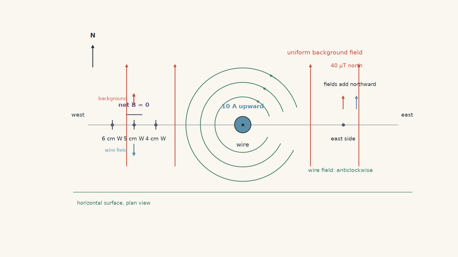
Determine:
- whether there is a point east or west of the wire where the net magnetic field is zero,
- the signed Hall-probe readings \(4.0\ \text{cm}\) west and \(6.0\ \text{cm}\) west of the wire, and
- what happens to the field direction as the probe passes through the zero-field point.
A student then says, “A magnetic field line must continue smoothly straight through that point because magnetic field lines never cross or stop.” Assess that statement.
Solution 5
There is one zero-field point \(5.0\ \text{cm}\) west of the wire, there is no corresponding zero east of the wire, and the net field reverses direction as the probe passes through the western zero. At the zero itself, \(\vec B=0\), so the magnetic-field direction is undefined.
On the western side of a wire carrying current upwards, the wire’s anticlockwise magnetic field points south. It therefore opposes the \(40\ \mu\text{T}\) northward background field.
For cancellation,
\[ B_{\text{wire}}=B_{\text{background}}. \]
Using
\[ B_{\text{wire}} =\frac{\mu_0 I}{2\pi r}, \]
we have
\[ 40\times10^{-6} = \frac{(4\pi\times10^{-7})(10)} {2\pi r}. \]
Since
\[ \frac{\mu_0 I}{2\pi} =2.0\times10^{-6}\ \text{T m}, \]
\[ r=\frac{2.0\times10^{-6}} {40\times10^{-6}} =0.050\ \text{m}. \]
Therefore,
\[ r=5.0\ \text{cm} \]
west of the wire.
On the eastern side, the wire’s field points north. It therefore adds to the northward background field rather than opposing it, so no zero occurs there.
At \(4.0\ \text{cm}\) west,
\[ \begin{aligned} B_{\text{wire}} &=\frac{2.0\times10^{-6}}{0.040}\\ &=50\ \mu\text{T}. \end{aligned} \]
This field points south, while the background field is \(40\ \mu\text{T}\) north. Taking north as positive,
\[ B_{\text{net}}=40-50=-10\ \mu\text{T}. \]
So the probe reads
\[ -10\ \mu\text{T}, \]
meaning \(10\ \mu\text{T}\) south.
At \(6.0\ \text{cm}\) west,
\[ \begin{aligned} B_{\text{wire}} &=\frac{2.0\times10^{-6}}{0.060}\\ &=33.3\ \mu\text{T}. \end{aligned} \]
Therefore,
\[ B_{\text{net}}=40-33.3 =+6.7\ \mu\text{T}. \]
The field now points north.
So, moving from \(4.0\ \text{cm}\) west to \(6.0\ \text{cm}\) west, the net field goes from southward, through zero at \(5.0\ \text{cm}\), to northward.
The student’s argument misses an important condition behind the usual field-line rules. At an ordinary point where \(B\neq0\), a field line has a unique tangent because the magnetic field has a unique direction. At the cancellation point, however,
\[ \vec B=0. \]
A zero vector has no direction. The ordinary instruction “draw the field line tangent to \(\vec B\)” therefore cannot define a unique direction at that exact point.
A careful field map would show a weak-field or null region around the cancellation point, with the surrounding field pattern changing as the competing fields take over. You cannot insist that one ordinary field line simply continues straight through the zero by applying a rule that assumes a non-zero field direction.
The tempting first answer is that both sources are producing magnetic fields, so some magnetic field must remain everywhere. The crucial constraint is vector superposition: two non-zero fields can produce a zero net field when they have equal magnitudes and opposite directions.
10What this lets you do next
Once you can move reliably between field-line diagrams and numerical values of \(B\), magnetic-force questions become much less mysterious.
The field-line model tells you which way the field points and how its strength changes through space. The quantitative model gives you the \(B\) value needed in equations such as \(F=BIL\sin\theta\) or \(F=qvB\sin\theta\).
That is the useful division of labour: the picture tells you what the field is doing, while the number tells you how strongly it can affect something placed in that field.